DiAna (under construction)


The development of DiAna, an acronym for Distortion Analyser, dates back to nineties. In those days spectrum analysers (or an 'AP') were expensice. So I wondered, whether it would be possible to do the same with a sound card together with appropriate software? In those days only a few sound cards were available and offered very limited capabilities. Nevertheless I started this project in the hope that I could compensate for these shortcomings by developing more elaborate software. BUT.........
I've suspended this project for the time being, because of lack of a decent sound card for accurate HD and IM measurements.
A Waveterminal X192 for example, even after extensive modifications, wasn't good enough.
(Too much Harmonic distortion at 20kHz as well as I.M. distortion between the channels due to stereo DACs and ADCs. Aargh!)
That was the status quo as of 2005 and further developments came to an halt during the next eight years.
In 2013 however, I stumbled on a few Lynx L22 sound cards on ebay, which were relative cheap. These cards are targeted at a professional market and are much better than any consumer product. So I resumed this project. As a result, their are currently two versions: one pro and one crippled demo version. The latter can be downloaded at www.data-odyssey.nl/diana/. The latest product version is 1.xx.xx After unzipping (of course) the executable can be installed anywhere on your hard disk, as it is a so called 'portable application'. I recommend to put it in a separate directory where also an ini and data files will be saved. Note that DiAna doesn't pollute your registry or whatsoever. Note that the zip file is password protected. Learn more at the bottom of this page.
At he moment, one important thing is still missing: documentation and help files. But in case of any question, please don't hesitate to contact me.
What is DiAna?
Apart from just an acronym for Distortion Analyzer, is it yet another software tool for analyzing distortions in audio amplifiers? Yes and No. Yes, because it measures the THD and IMD spectrum as well as the frequency response just like many other software tools are capable of doing this. No, because it also can detect spectrum components, which are solely related to the fundamental frequency (i.e. harmonics), even if they are deeply burried in noise.
In addition, it also shows the residual, which is very convenient when, for example, optimizing the quiet current of a class B (or AB) output stage. A more unique feature is that it can measure harmonics far beyond the Nyquist frequency. Of course, this only makes sense if the ADC doesnt cut-off these harmonics. A SAR-ADC with a wide band front-end can do this, while common audio ADCs will rigorously cut-off anything above the Nyquist frequency.
A few hints to get started:
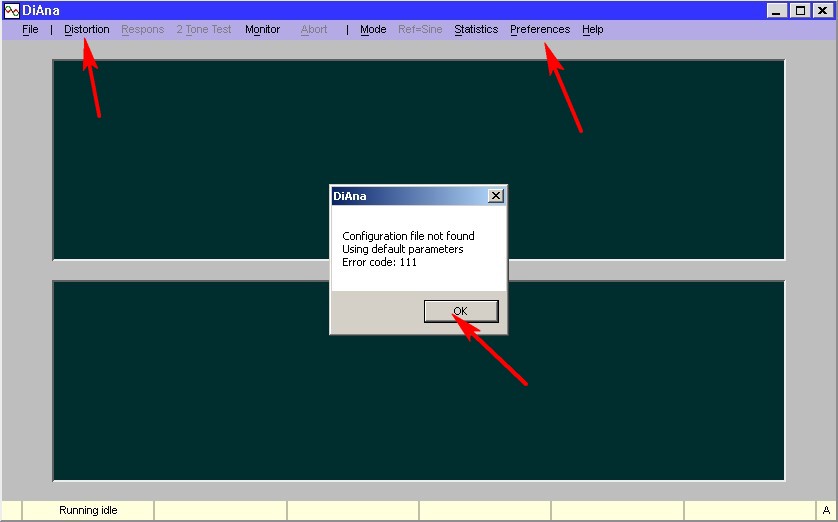
First, unzip the filer, of course, and put it in a separate directory. Since DiAna is a "portable" application, you can put it anywhere on your disk. Then, for a loop-back test, wire the sound card accordingly. After the very first start-up, you will get an error message. It simply means that the ini file wasn't yet present, so don't worry. Just press OK or ESC to remove the message.
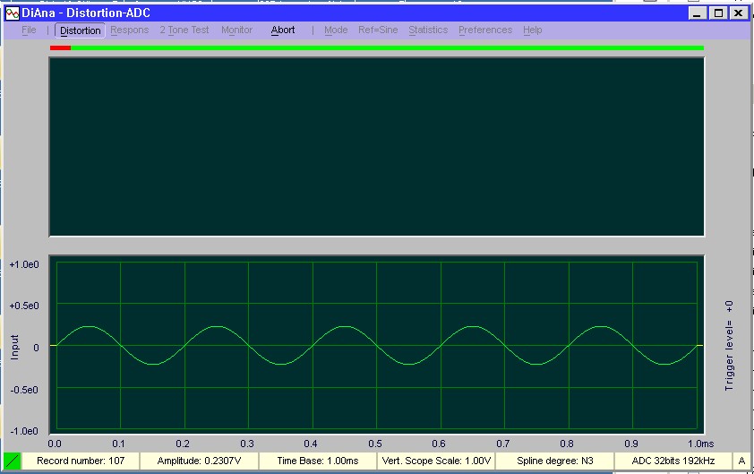
Next, click on the Distortion button. If every thing went well the program starts collecting data during 2.5 seconds (100 records). In the lower pane the input signal is displayed
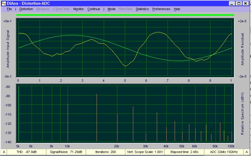
When done the THD spectrum in the lower pane is shown, while in the upper pane the input signal and the so called residual is shown.
But maybe it didn't go that easy. During start-up for example, the first detected ASIO is selected. Suppose this one wasn't wired for loop-back at all, then you don't get a signal, of course. In that case go to Preferences->Sound card and select the right sound card. Hereafter this one will be selected automatically.
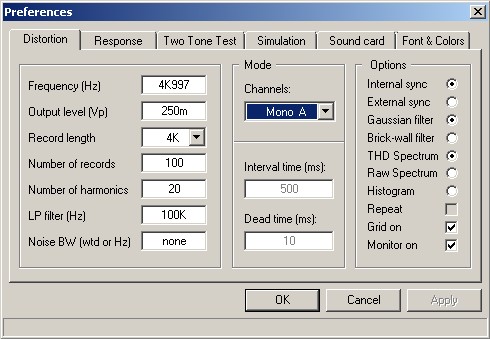
To select another frequency, amplitude, spectrum or whatsoever, go to Preference->Distortion
Under de hood:
In order to use this tool, one should have a basic understanding of how DiAna works, in particular with respect to choosing the right record length. Instead of collecting and averaging the stream of input data in a single run, this data stream is subdivided over a number of records. In doing so, the effect of possible amplitude and offset drift will be minimized. The shorter the records size, the shorter the influence of drift. On the other hand however, each records should contain enough information to accurately determine amplitude, frequency, phase and offset of the fundamental. These variables are needed in the next averaging step. So each record should span at least say three cycles. Regarding the number of records, the more available, the better the suppression of noise and hum effects on the final THD spectrum. In general, a total measuring time of about 10 seconds will give satisfactory results. After further analysis, the results are displayed graphically as well as numerical.
Averaging.
Input samples are mapped into a fixed interval, ranging from 0 to 2pi (by means of modulo 2pi arithmetic).
In order to make this stream of data manageable, this interval is subdivided in 1024 bins (actually an array 1024 x 80 bits) and each sample, after the fundamental has been subtracted (leaving only the residual), is accumulated in one of these bins. Clearly, the phase of a samples could have any value between 0 and 2pi, but since they are categorized in limited number (1024) of discrete values, giving rise to a sort of round off errors. How to deal with that will be discussed later on. After all data are collected, the residual is normalized by dividing the content of each bin by the numbers of samples stored in it. Bins might be empty, in which case these gaps are filled by means of interpolation, to be more precisely, by means of a periodic cubic spline.Gaps arise when the sampling frequency (fs) is a whole and relative small multiple of the signal frequency (fi), e.g. 192kHz respectively 4kHz. They seldom give rise to problems, but it is better to avoid them anyhow. In such case one should choose something like 3.999kHz or 4.001kHz.Now, we have the residual in its raw form. It should noted that the bandwidth of the residual is essentially not limited by the Nyquist frequency (fs/2) but the fundamental frequency times half the number of bins (fi x 512), unless the ADC is provided with an anti-alias filter as limiting factor (sound-card always has such filter).
Therefore, the spectrum at higher frequencies might look rather noisy and it is desirable to filter it out.
In order to subtract the fundamental, the exactly the amplitude, offset and phase of the fundamental have to been known. When the DAC and ADC are not synchronized or an external signal source is used, also the exact frequency has to be determined. in this case, select "External sync" to enable the frequency discrimator. In case DAC and ADC are synchronized, select "Internal sync". The latter mode is faster and less computation-intensive.
As these parameters slightly vary over time, averaging the data in a single run is not a good idea. Therefore, averaging is done over small chunks (records of say 4096 samples) and the results summed together.
Noise measurement.
Noise is measured by calculating THD+N first and then later on subtracting THD from it.
Although the THD measurement is extreme sensitive, as low as -300dB, it is not extreme accurate, only some 5 to 6 digits, mainly depending on the re-sampling and interpolating process. On the other hand, THD+N is calculated by subtracting a sine directly from the input samples without any further hassle (except low-pass filtering).Obviously, subtracting THD from THD+N will not give the exact answer. In case the actual noise is zero or far below the THD level, even a negative figure can result (you can check this by simulation: negative noise is indicated by an trailing * (e.g. -187dB*).Regarding real life signals, the noise level is probably of the same order as THD and the 'gross' inaccuracy, as outlined above, is completely masked.The noise bandwidth has to be specified, of course, otherwise the measurement is meaningless. The bandwidth can be specified in the Distortion Preference Menu: in Hz or A, B or C-weighting. If none is specified (i.e. zero), the bandwidth is limited to the Nyquist frequency.
One more important thing: The right mouse button is your best friend, as a lot more pop-up menus can invoked with this button.
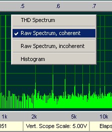
To switch between different kinds of spectra, THD, Raw, etc.: Click with the right mouse button on the lower pane.
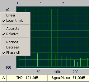
To switch between Relative Spectrum and Absolute Spectrum: Click with the right mouse button on the lower left border.
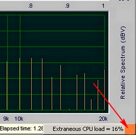
When the small square at the lower left corner lights up, orange for warning, red for error, right click on this square to see what's wrong. In this example the CPU was for 16% busy with other things, which DiAna doesn't like. Left click on this square to clear the message. Also, there are a lot of keyboard short cuts. This will be covered later in more detail.
Additional information can be found here:
http://www.diyaudio.com/forums/equipment-and-tools/315785-diana-software-distortion-analyzer-post5266519.html
For those who experience troubles with E-MU sound card drivers under Windows-10, please visit this site:
https://www.kvraudio.com/forum/viewtopic.php?t=529349
Virus:
Please, be aware that some anti virus scanners will identify DiAna as dangerous. This is a 'false positive'. Just ignore it. Remember, no software is 100% perfect and that also applies to AV scanners.
In order to protect the zip file from possible attaks by evil people and also to avoid whining about supposed virus by companies like Netcraft, this file has been password protected. Just contact me via diyaudio.com to get the password for unzipping the file.
Right click on the lower pane
Right click on the lower left border
Right click on the error/warning square
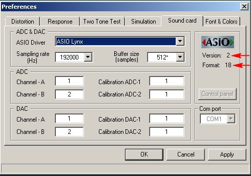
Sound card channel selection
DiAna supports two (stereo) channels, 'numbered' A and B. As most sound cards also have two channels, just assign channel A to the first sound card channel, i.e. #1 and channel B to the second one, i.e. #2, see the figure below. In case the sound card have more channels, you are free to use some other channels. This applies to the ADC as well to the DAC.
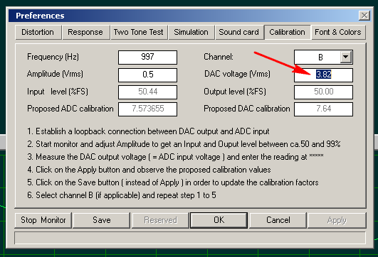
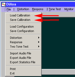
Sound card calibration
In essence, the ADC and DAC calibration fields of the Sound card menu should be filled in with the full scale input rms voltage of the ADC respectively the full scale output rms voltage of the DAC. This can be done in two ways: either manual or semi-automatic. In both cases, create a loop back connection between ADC and DAC and also attach an external voltmeter to it, either calibrated in V-RMS or dbV.
First, let's go on with the manual procedure for channel A.
1. In the Sound card menu set all four Calibration factors to 1Vrms
2. In the Distortion menu: set Data channels to stereo A & B and ref. channel to none.
3. In the same menu set Frequency to some convenient value, for example 997Hz and the Output level to 1Vrms
4. Start the Monitor function.
5. Measure the DAC-A output voltage with the external voltmeter and store the reading at DAC Calibration-A.
6. Select the %-FS mode in the Amplitude pan of the status bar.
7. Adjust the Output level in such a way to get an Amplitude as close as possible of 100%.
8. Measure the ADC-A input voltage (same as DAC-A output voltage, of course) and store the reading at ADC Calibration-A.
9. Repeat above steps from 2 to 8 for channel B.
With a Lynx L22 sound card set at +4dBu levels, I measure 7.77Vrms in step 5 and 7.71Vrms in step 8
The semi-automatic procedure requires a few less steps. Moreover, it doesn't need a reset of the calibration factors to 1Vrms, as other values are automatically taken into account. Just press the Calibration button in the menu bar and follow the steps as shown by the program itself.
How different calibration settings can be saved and retrieved.
Characterizing a notch filter
Standard procedure:
Filter characterization is rather simple. Connect the sound card in loopback mode. One channel (used as reference) directly and the other (test) channel via the notch filter. In the Distortion menu select the Ref. channel accordingly. Also, select in the Option menu 'Characterize notch filter'.
Now run a "distortion" measurement for say 100 records and save the result under File->Save Notch Filter.
In order to use the saved data, run a distortion measurement as usual and select in the Option menu Apply notch compensation, which takes care of the amplitude and phase correction of the harmonics.
Extended procedure:
1. Connect the sound card in loopback mode. One channel directly (the reference channel) and the other channel via the notch filter (the test channel) .
2. In the Distortion menu select which channel is used as reference.
3. Select in the Option menu 'Characterize notch filter'.
4. Now run the first measurement for say 100 records by pressing the Distortion button.
5. When finished, don't save the result yet. Instead, exchange the channels, i.e. connect the notch filter to the other channel
6. In the Distortion menu set the reference channel accordingly.
7. Start the second run by pressing the Continue button.
8. When finished, go to File->Save Notch Filter and save the result as usual
The difference with the standard procedure is that inter channels imbalances, in terms of gain and phase, are averaged out and errors are hopefully reduced to zero.
NB: No interpolation has been applied to compensate for mismatches (if any) between harmonics as saved in the notch file and harmonics of subsequent THD measurements. So ensure to use the correct and same fundamental frequency, which matches the notch filter itself, the characterization file and THD measurements.
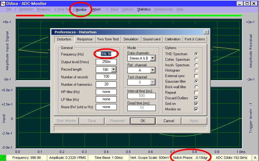
How to find the exact notch frequency?
Connect the notch filter as outlined above, select the correct reference channel, select 'Characterize notch filter' option, open the Distortion menu and click on the Monitor button. The phase difference between 'notched' signal and reference signal is displayed on the status bar. While running, now you can change the frequency 'on the fly' in order the minimize the phase (see picture below).